library(SamplingDesignTools)
library(survival)
library(dplyr)
##
## Attaching package: 'dplyr'
## The following objects are masked from 'package:stats':
##
##     filter, lag
## The following objects are masked from 'package:base':
##
##     intersect, setdiff, setequal, union
library(knitr)
data("cohort_1")4 Weighted analysis of (more) extreme case-control samples
4.1 Method overview
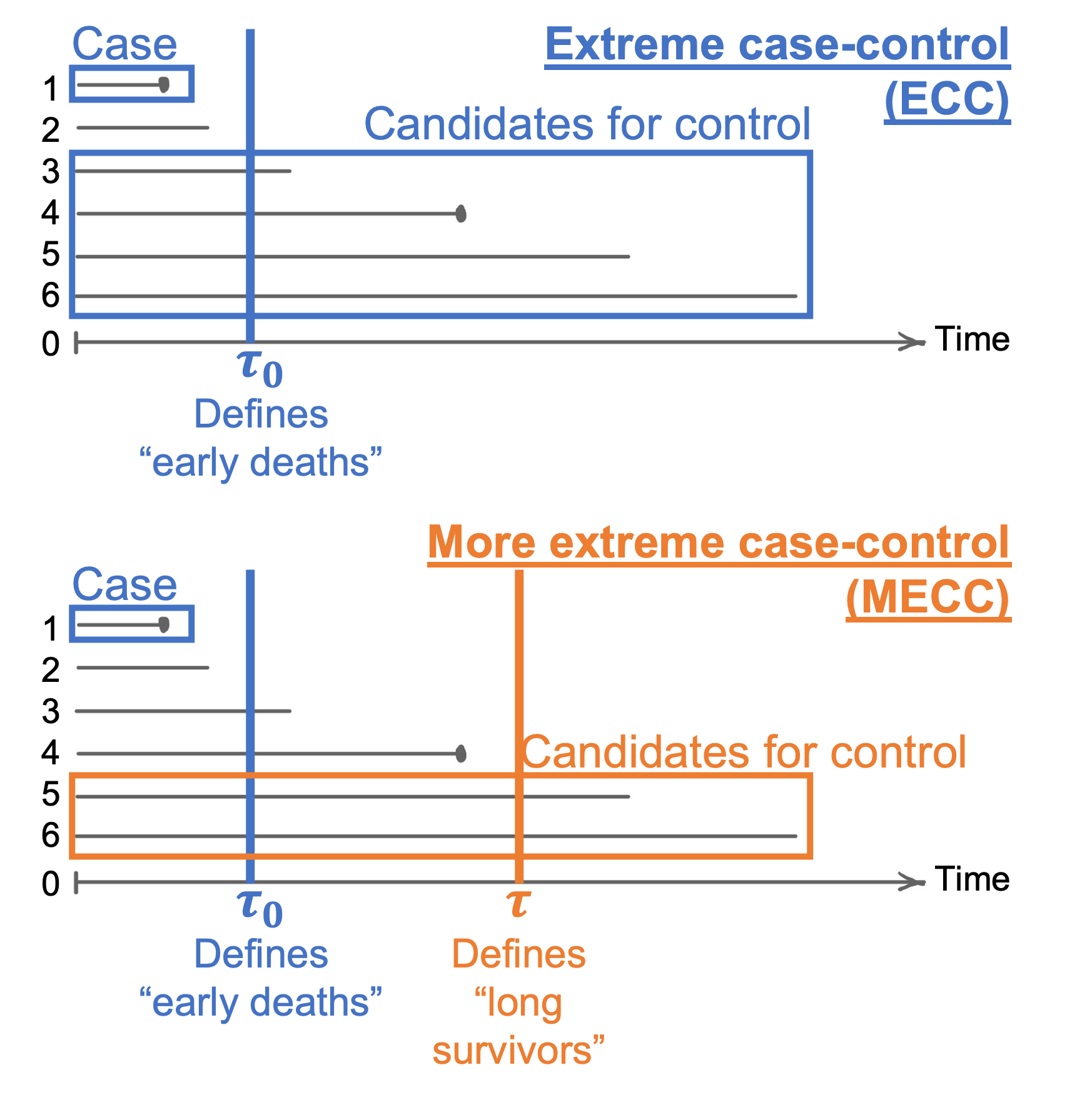
An extreme case-control (ECC) study is only interested in “early deaths” design, and a more extreme case-control (MECC) further restricts candidate controls to “longer survivors”. These two types of study designs are described in the figure below.
This section illustrates the weighted analysis of MECC samples using the conditional approach described in Section 2.2 of Salim et al (2014), using the simulated cohort described in Section 1 of this paper:
- Salim A, Ma X, Fall K, Andrén O, Reilly M. Analysis of incidence and prognosis from ‘extreme’ case‐control designs. Statistics in medicine. 2014 Dec 30;33(30):5388-98.
4.2 Load packages and data
The example in this section uses cohort_1 as the underlying cohort.
4.3 1:2 MECC matched on gender
For illustrative purpose, a MECC sample was drawn by frequency-matching 2 controls to each case on gender. “Early deaths” were defined as events before \(\tau_0 = 5\) years of follow-up, and “long survivors” were defined as subjects who did not have the event in the first \(\tau = 15\) years of follow-up. Note that an event in a MECC study (y_mecc) has a different definition as an event in the original cohort study.
set.seed(1)
dat_mecc <- draw_mecc(cohort = cohort_1, tau0 = 5, tau = 15,
                      id_name = "id", t_name = "t", delta_name = "y",
                      match_var_names = "gender", n_per_case = 2)
## Joining, by = "gender"
## Joining, by = c(".t", ".strata")
## Joining, by = ".strata"
kable(head(dat_mecc))| id | y | t | age | gender | y_mecc | surv | surv_tau | set_id_mecc |
|---|---|---|---|---|---|---|---|---|
| 8756 | 1 | 2.1351357 | 76 | 0 | 1 | 0.9943501 | 0.957786 | set_8756 |
| 8069 | 1 | 3.6774974 | 74 | 0 | 1 | 0.9898270 | 0.957786 | set_8069 |
| 5939 | 1 | 0.8364486 | 49 | 0 | 1 | 0.9979733 | 0.957786 | set_5939 |
| 1756 | 1 | 4.3993170 | 63 | 0 | 1 | 0.9878869 | 0.957786 | set_1756 |
| 7955 | 1 | 4.4904526 | 64 | 0 | 1 | 0.9876400 | 0.957786 | set_7955 |
| 1531 | 1 | 2.5664238 | 69 | 0 | 1 | 0.9918995 | 0.957786 | set_1531 |
table(y = dat_mecc$y, y_mecc = dat_mecc$y_mecc)
##    y_mecc
## y     0   1
##   0 397   0
##   1  11 204
As the conditional analysis of the MECC sample assumes individual matching, the function draw_mecc randomly matches controls to each case to form matched sets, indicated by the variable set_id_mecc. In addition, this function provides the estimated baseline survival probabilities (i.e., \(\hat{S}(t_i)\) and \(\hat{S}(\tau)\)) that are needed to compute the weighted likelihood.
The weighted approach estimates the HR, where all covariates need to be centred at the cohort average:
dat_mecc$age_c <- dat_mecc$age - mean(cohort_1$age)
# When there is only a single coefficient in, users should provide reasonable
# lower and upper limits for the estimate:
m_mecc <- analyse_mecc_cond(
  y_name = "y_mecc", x_formula = ~ age_c, set_id_name = "set_id_mecc",
  surv = dat_mecc$surv, surv_tau = dat_mecc$surv_tau, mecc = dat_mecc,
  lower = -1, upper = 1
)
## Warning in optimize(function(par) fn(par, ...)/con$fnscale, lower = lower, : NA/
## Inf replaced by maximum positive value

## Warning in optimize(function(par) fn(par, ...)/con$fnscale, lower = lower, : NA/
## Inf replaced by maximum positive value
round(m_mecc$coef_mat[, -1], 3)
##        est exp_est   se pval
## age_c 0.11   1.116 0.01    0
4.4 Compare results
coef_cox_cohort_1 <- summary(m_cox_cohort_1)$coef
kable(data.frame(
  Data = c("Full cohort", "1:2 MECC, weighted"),
  Variable = "Age",
  `True HR` = 1.1,
  `Estimated HR` = c(coef_cox_cohort_1["age", "exp(coef)"],
                     m_mecc$coef_mat["age_c", "exp_est"]),
  `SE of log(HR)` = c(coef_cox_cohort_1["age", "se(coef)"],
                     m_mecc$coef_mat["age_c", "se"]),
  `p-value` = c(coef_cox_cohort_1["age", "Pr(>|z|)"],
                     m_mecc$coef_mat["age_c", "pval"]),
  check.names = FALSE
), digits = c(0, 0, 1, 2, 3, 3))| Data | Variable | True HR | Estimated HR | SE of log(HR) | p-value |
|---|---|---|---|---|---|
| Full cohort | Age | 1.1 | 1.11 | 0.004 | 0 |
| 1:2 MECC, weighted | Age | 1.1 | 1.12 | 0.010 | 0 |